Welcome to technical page
CLT with MATLAB <= |
Invariant theory |
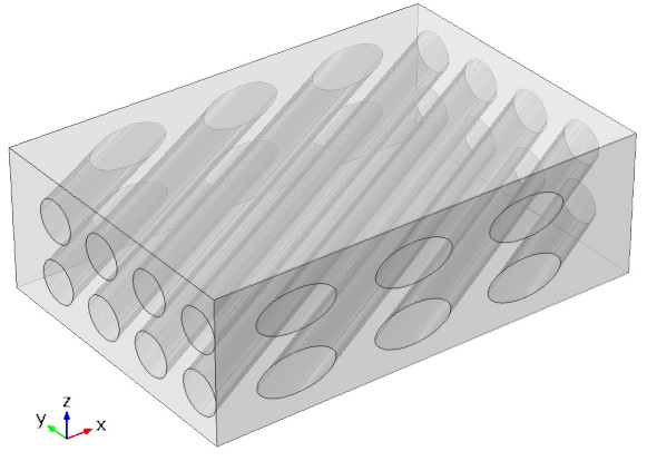
Marine turbine |
Statistics |
Classical laminate theory
This page gives the formulae of classical laminate theory and its implementation in MATLAB platform.
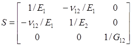
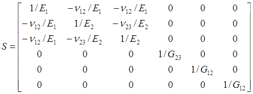
1, Composite lamina: a kind of orthotropic material

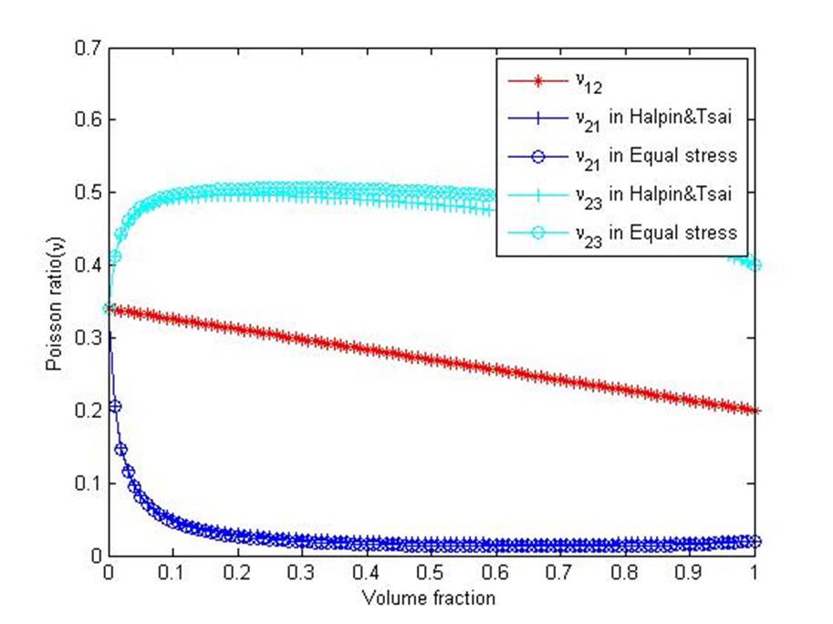
The longitudinal elastic modulus and in-plane Poisson’s ratio are calculated by the fibre volume fraction,
![]()
![]()
The Poisson’s ratio various to fibre volume fraction look like this,
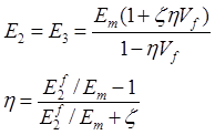
The transverse modulus, out-off plane modulus and in-plane shear modulus are calculated by an empirical equation, called Halpin-Tsai equation (Halpin and Kardos 1976),
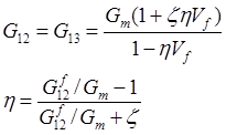
The transverse Poisson’s ratio is calculated by this equation which is derived from a hydrostatic assumption (Meng 2015),
And then the last elastic component, transverse shear modulus is obtained,
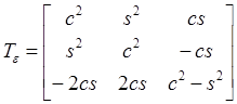
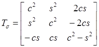
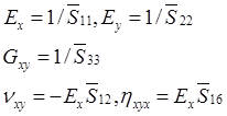
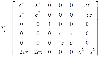
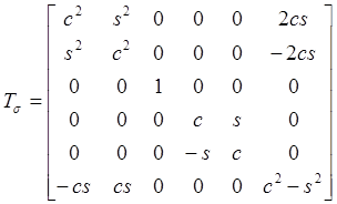
2, Off-axis lamina: the coordinate system (x,y,z) has a rotational angle to the original system (1,2,3)
For the 2D version of stress tensor transformation (Hull and Clyne 1996),
![]()
![]()
There is a new element in the off-axis compliance matrix (called as interaction ratio),![]() which is usually nonzero. It represents the ratio of the shear strain
which is usually nonzero. It represents the ratio of the shear strain ![]() induced by normal stress
induced by normal stress ![]() to the normal strain
to the normal strain![]() induced by the same normal stress
induced by the same normal stress![]() . The interaction ratio various to rotational angle look like this,
. The interaction ratio various to rotational angle look like this,
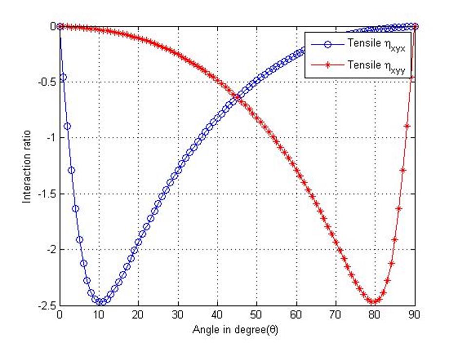
The minimum value of interactional ratio appears around 11 ̊. It is interesting to find that, for most of the CFRP composites, this value falls in the range of 10 ̊-13 ̊ with very small standard deviation (Meng, 2015).
For the 3D version of stress tensor transformation, a 3D stress tensor transformation matrix is introduced (Lekhnitskiĭ 1963),
3, Composite laminate: a stack of composite laminas which are bonded to provide required engineering properties
The compliance matrix should be calculated by the stiffness matrix first,
![]()
Substituting the composites compliance matrix into CLT equations (Kaw 2006),
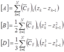
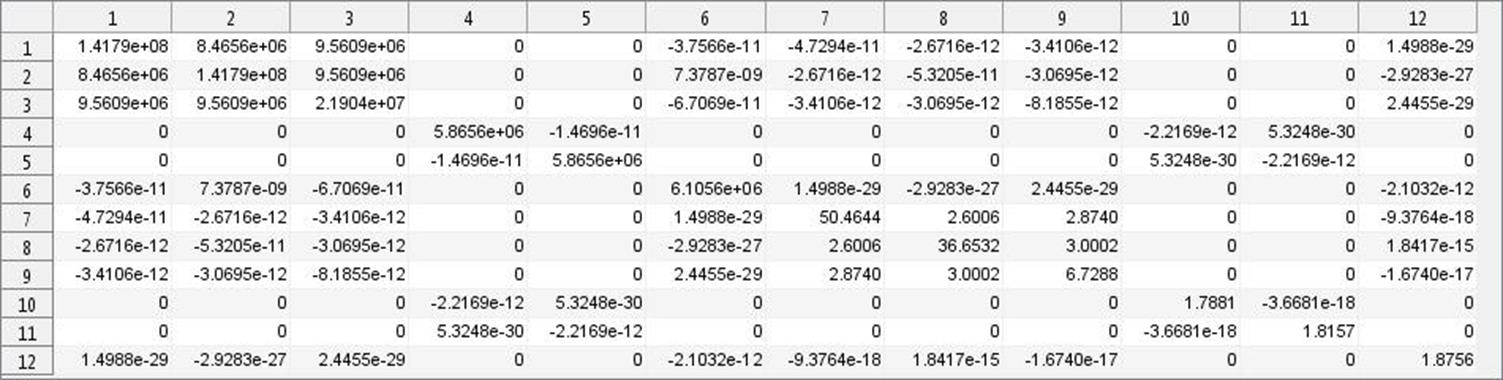
Assembling the [A], [B] and [D] matrices for  matrix, and its inversed
  matrix,
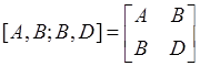
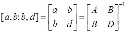
A typical [A,B;B,D] matrix look like this ([0/90]s laminate),
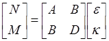
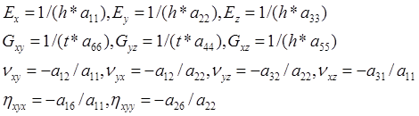
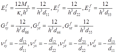
Once the ![]() matrix is assembled, the elastic properties of laminate can be evaluated by (Kaw 2006)
matrix is assembled, the elastic properties of laminate can be evaluated by (Kaw 2006)
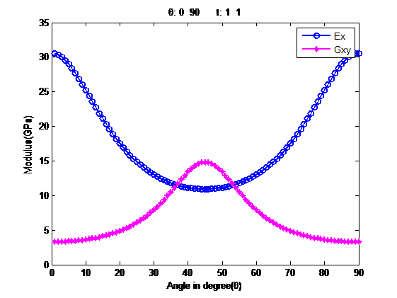
With these CLT formulae, it is possible to predict the elastic properties in any rotational angle. For a very simple cross-ply laminate, say [0/90] stacking, its Young’s modulus and shear modulus various to rotated angle (theta) look like this,
The above formulae are derived for the tensile properties, however the flexural properties are different.
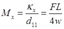
Consider a composite laminate with symmetric lay-up under three-point bending. The coupling matrix ![]() , so the moment about x axes can be written as,
, so the moment about x axes can be written as,
If it is assumed that the curvature through-thickness is a constant, the strain and longitudinal stress are determined by,
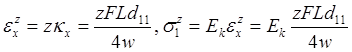
and the apparent flexural properties (Kaw 2006),
The maximum strain appears on the top and bottom surfaces![]() . However, the maximum stress is dependent on both the through-thickness coordinate and the ply modulus.
. However, the maximum stress is dependent on both the through-thickness coordinate and the ply modulus.
With the 3D version of ![]() matrix, the interlaminar shear stress
matrix, the interlaminar shear stress ![]() and transverse shear stress
and transverse shear stress ![]() can be evaluated by the principle of continuum mechanics (Creemers 2009),
can be evaluated by the principle of continuum mechanics (Creemers 2009),
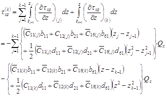
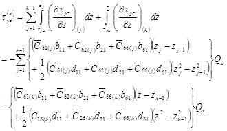
The local interlaminar shear stress in the ![]() ply (along fibre orientation) is evaluated according to its orientation,
ply (along fibre orientation) is evaluated according to its orientation,
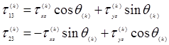
For an angle-ply laminate ([±45]s)subjected to 3-point bending, its interlaminar shear stress along thickness direction distributes like this,
4, Implementation in MATLAB
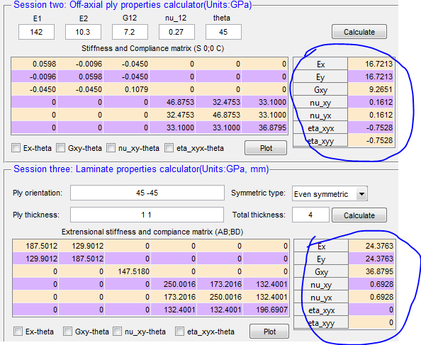
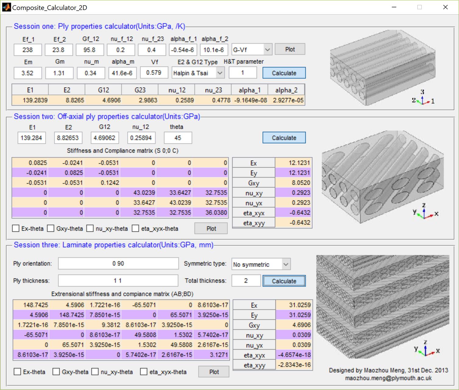
These CLT formulae can be solved by MATLAB. To download this MATLAB code, please click here (if you can not download it, try to right-click and copy the address to IE explorer). This figure gives the GUI of the MATLAB tool.
5, Validation
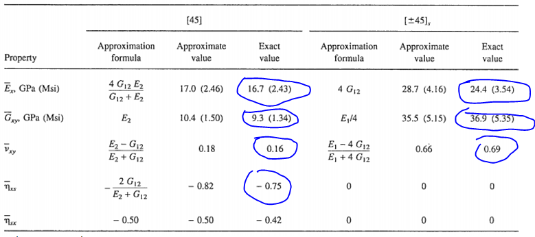
In the book “Engineering Mechanics of Composite Materials”, Daniel and Ishai gave overall laminate properties for [45] ply and a [![]() 45]s made of Carbon/Epoxy (AS4/3501-6, E1 = 142GPa, E2 = 10.3GPa, G12 = 7.2GPa, and ν12 = 0.27). The results are given in the following table. And the results calculated by this MATLAB tool are also given for comparison.
45]s made of Carbon/Epoxy (AS4/3501-6, E1 = 142GPa, E2 = 10.3GPa, G12 = 7.2GPa, and ν12 = 0.27). The results are given in the following table. And the results calculated by this MATLAB tool are also given for comparison.